SmoothSpline
SmoothSpline is a Matlab program for obtaining the best-fit smoothing spline to a set of noisy y(x) data. This spline is "best" in the sense that it has the minimum possible error, while still having minimal roughness. SmoothSpline is particularly useful for determining the derivatives (dy/dx, d^2y/dx^2, …) of noisy data, which cannot be obtained accurately otherwise.
License:
SmoothSpline is released under the GNU General Public License.
By downloading this software, you agree to abide by the GNU GPL conditions.
The most important conditions are as follows:You may copy, modify, and redistribute the software freely.
Any such redistributions must be done under the terms of the GPL.
Software:
smoothspline7.zip — SmoothSplne 7.0 source code (requires Matlab Curve Fitting Toolbox)
Author: Brenden Epps
Documents:
Epps MME 2010 conference presentation: PDF
Double bisection method illustration: PDF
Reference:
B.P. Epps, T.T. Truscott, and A.H. Techet, "Evaluating derivatives of experimental data using smoothing splines," Mathematical Methods in Engineering International Symposium, Coimbra, Portugal, October 2010. PDF
T.T. Truscott, B.P. Epps, and A.H. Techet, "Unsteady forces on spheres during free-surface water entry," Journal of Fluid Mechanics, vol. 704, 2012, pp. 173-210. HTML PDF ResearchGate
For additional references, see citing articles in Google Scholar.
For additional information, see SmoothSpline on the MathWorks File Exchange.
Example
Consider the forces acting on a billiard ball falling into a pool of water. Since force = mass*acceleration, we need to know the acceleration of the ball — however, only the position y(t) can be measured directly from the high-speed video images. The acceleration (and hence the force) must be obtained from the second derivative of the measured data: a(t) = d^2y/dt^2.

A billiard ball falls into a quiescent pool of water. Position, y, is measured in each timestep, t, by inspection of the images.
SmoothSpline is used to fit a series of smoothing splines to the digitized position data. Observe the elbow in the Roughness-versus-Error-tolerance plot; the selected spline has the minimum error possible while still having minimal roughness.
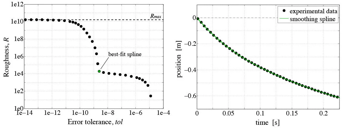
(left) “Efficient frontier” of roughness versus error tolerance of a series of smoothing splines. (right) Position data and spline fit.
The second derivative of the position data can be determined most accurately using the smoothing spline. Local (windowed) least squares provides a good estimate of the derivative, but it is not guaranteed to be smooth. Polynomial fits to the entire data set yield poor predictions of the derivative. Finite difference methods are horribly inaccurate, because they amplify the noise in the data.
